
A chord diagram in R
A chord diagram is a graphical representation of the data in a matrix’s interrelationships. The data is arranged in a radial pattern around a circle, with the relationships between the data points commonly depicted as arcs linking the dots (Wikipedia). Each entity is represented by a fragment on the outer part of the circular layout. Then, arcs are drawn between each entities. The size of the arc is proportional to the importance of the flow.
Using the htmlwidgets interface architecture, the chorddiag package in R allows us to build interactive chord diagrams using the JavaScript visualization library D3 from within R.
We’ll look at how to make interactive chord diagrams in this blog post. You can view how many regions from each environmental challenges are by hovering over the arcs for each region/section below.
require(tidyverse)
require(viridis)
require(chorddiag)  #devtools::install_github("mattflor/chorddiag")
We create a dataframe of four regions in Tanzania with with a count of people responded to the causes of environmental challenges
regions = data.frame(Mwanza = c(50, 25, 5, 12),
                      Dar = c(10, 55, 5, 20),
                      Tanga = c(45,12,29, 20),
                      Arusha = c(24,67,27,15))

regions
Mwanza Dar Tanga Arusha
1 50 10 45 24
2 25 55 12 67
3 5 5 29 27
4 12 20 20 15We then convert the region data frame to matrix and assign the corresponding environmental challenges as row names
regions = as.matrix(regions)
row.names(regions) = c("Climate", "Waste", "Pollution", "Deforestation")
We can then plot the chord diagram
regions %>% chorddiag(type = "bipartite",
                      showTicks = F,
                      groupnameFontsize = 14,
                      groupnamePadding = 10,
                      margin = 90, showGroupnames = T)
Sometimes we might not be interested with default colors and wish to define our own colors. Since we have four groups, let’s define the color and use it to make similar plot but with a different flavour from the color
groupColors <- c("#000000", "#FFDD89", "#957244", "#F26223")

regions %>% chorddiag(type = "bipartite",
                      showTicks = F,
                      groupColors = groupColors,
                      groupnameFontsize = 14,
                      groupnamePadding = 10,
                      margin = 90,
                      showGroupnames = T)
Chord diagrams can also be used to show transition matrices. Let’s pretend that each row in the dummy data below represents the number of customers each company has this year. Let’s imagine, though, that some of your clients decide to switch firms next year (shown in the columns). You may hover your mouse over the visualization to check which companies are losing the most clients and which are keeping the most.
df = data_frame(`Company A` = c(800, 200, 100, 50, 140, 200, 140),
                `Company B` = c(100, 2000, 300, 400, 50, 0, 290),
                `Company C` = c(200, 500, 4000, 80, 120, 320, 600),
                `Company D` = c(500, 200, 300, 5000, 250, 140, 450),
                `Company E` = c(600, 300, 150, 600, 6000, 30, 0),
                `Company F` = c(500, 400, 100, 300, 250, 4500, 140),
                `Company G` = c(300, 50, 0, 150, 600, 250, 7000))
df
# A tibble: 7 x 7
`Company A` `Company B` `Company C` `Company D` `Company E` Company ~1 Compa~2
<dbl> <dbl> <dbl> <dbl> <dbl> <dbl> <dbl>
1 800 100 200 500 600 500 300
2 200 2000 500 200 300 400 50
3 100 300 4000 300 150 100 0
4 50 400 80 5000 600 300 150
5 140 50 120 250 6000 250 600
6 200 0 320 140 30 4500 250
7 140 290 600 450 0 140 7000
# ... with abbreviated variable names 1: `Company F`, 2: `Company G`df = as.matrix(df)
row.names(df) = c(colnames(df))chorddiag(data = df,
type = "directional",
showTicks = F,
groupnameFontsize = 14,
groupnamePadding = 10,
margin = 90)Bonus
The bonus in this post is the chord diagram using dataset of estimates of global bilateral migration Flows by Gender between 1960 and 2015 published by Gui J. Abel
# Load dataset from github
data <- read.table("https://raw.githubusercontent.com/holtzy/data_to_viz/master/Example_dataset/13_AdjacencyDirectedWeighted.csv", header=TRUE)
# short names
colnames(data) <- c("Africa", "East Asia", "Europe", "Latin Ame.", "North Ame.", "Oceania", "South Asia", "South East Asia", "Soviet Union", "West.Asia")
rownames(data) <- colnames(data)mycolor <- viridis(10, alpha = 1, begin = 0, end = 1, option = "D")
data %>%
as.matrix() %>%
chorddiag(type = "directional",
showTicks = F, groupColors = mycolor,
groupnameFontsize = 14,
groupnamePadding = 10,
margin = 90)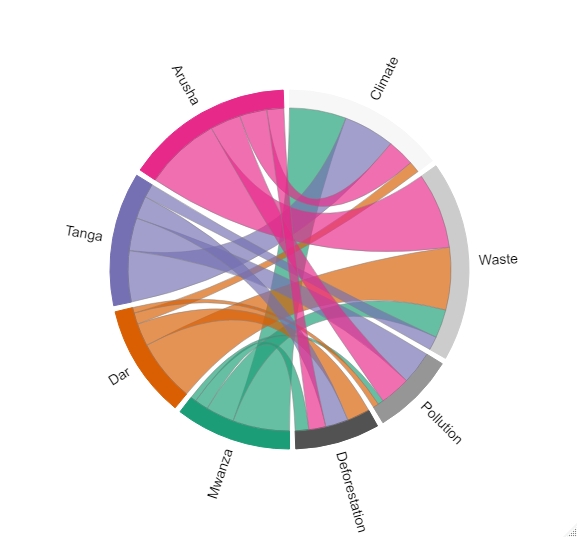
Figure 1: leo
