Open Street Map Data in R
OpenStreetMap is a collaborative project to create a free editable geographic database of the world. Open street Map (OSM) is name refer is a global open access mapping project. The data from OSM can be used in various ways including production of paper maps and electronic maps, geocoding of address and place names, and route planning.
To easy access of OSM spatial data, Mark Padgham and Robin Lovelace developed osmdata, which is an R package for downloading data from OSM. This tutorial takes you through the steps of retrieving points of interest in defined geographical areas using the osmdata package, and visualising them using the ggmap and ggplot2 packages.
We can install and load the osmdata package from CRAN as follows
install.packages("osmdata")Before we explore the package, Once installed into the machine, we load the packages we need for this session as follows
require(osmdata)
require(sf)
require(ggmap)
require(tidyverse)
require(patchwork)
Exploring the osmdata package
The osmdata package provides spatial data about a wide range of spatial properties and objects across the world. The available_features() function can be used to get the list of recognized features in OSM. A list of the available features can be found in the OSM wiki.
available_features() [1] "4wd_only" "abandoned"
[3] "abutters" "access"
[5] "addr" "addr:city"
[7] "addr:conscriptionnumber" "addr:country"
[9] "addr:district" "addr:flats"
[11] "addr:full" "addr:hamlet"
[13] "addr:housename" "addr:housenumber"
[15] "addr:inclusion" "addr:interpolation"
[17] "addr:place" "addr:postbox"
[19] "addr:postcode" "addr:province"
[21] "addr:state" "addr:street"
[23] "addr:subdistrict" "addr:suburb"
[25] "admin_level" "aeroway"
[27] "agricultural" "alt_name"
[29] "amenity" "area"
[31] "atv" "backward"
[33] "barrier" "basin"
[35] "bdouble" "bicycle"
[37] "bicycle_road" "biergarten"
[39] "boat" "border_type"
[41] "boundary" "bridge"
[43] "building" "building:fireproof"
[45] "building:flats" "building:levels"
[47] "building:min_level" "building:soft_storey"
[49] "bus_bay" "busway"
[51] "charge" "construction"
[53] "construction#Railways" "covered"
[55] "craft" "crossing"
[57] "crossing:island" "cuisine"
[59] "cutting" "cycleway"
[61] "denomination" "destination"
[63] "diet" "diplomatic"
[65] "direction" "dispensing"
[67] "disused" "disused:shop"
[69] "drive_in" "drive_through"
[71] "ele" "electric_bicycle"
[73] "electrified" "embankment"
[75] "embedded_rails" "emergency"
[77] "end_date" "entrance"
[79] "est_width" "fee"
[81] "fire_object:type" "fire_operator"
[83] "fire_rank" "foot"
[85] "footway" "ford"
[87] "forestry" "forward"
[89] "frequency" "fuel"
[91] "gauge" "golf_cart"
[93] "goods" "hazmat"
[95] "healthcare" "healthcare:counselling"
[97] "healthcare:speciality" "height"
[99] "hgv" "highway"
[101] "historic" "horse"
[103] "ice_road" "incline"
[105] "industrial" "inline_skates"
[107] "inscription" "internet_access"
[109] "junction" "kerb"
[111] "landuse" "lanes"
[113] "lanes:bus" "lanes:psv"
[115] "layer" "leaf_cycle"
[117] "leaf_type" "leisure"
[119] "lhv" "lit"
[121] "location" "man_made"
[123] "maxaxleload" "maxheight"
[125] "maxlength" "maxspeed"
[127] "maxstay" "maxweight"
[129] "maxwidth" "military"
[131] "minspeed" "mofa"
[133] "moped" "motor_vehicle"
[135] "motorboat" "motorcar"
[137] "motorcycle" "motorroad"
[139] "mountain_pass" "mtb:description"
[141] "mtb:scale:imba" "mtb_scale"
[143] "name" "name:left"
[145] "name:right" "narrow"
[147] "natural" "noexit"
[149] "non_existent_levels" "note"
[151] "nudism" "office"
[153] "official_name" "old_name"
[155] "oneway" "opening_hours"
[157] "operator" "organic"
[159] "oven" "overtaking"
[161] "parking:condition" "parking:lane"
[163] "passing_places" "place"
[165] "power" "priority_road"
[167] "produce" "proposed"
[169] "protected_area" "psv"
[171] "public_transport" "railway"
[173] "railway:preserved" "railway:track_ref"
[175] "recycling_type" "ref"
[177] "religion" "residential"
[179] "roadtrain" "route"
[181] "sac_scale" "service"
[183] "service_times" "shelter_type"
[185] "shop" "short_name"
[187] "sidewalk" "site"
[189] "ski" "smoothness"
[191] "social_facility" "sorting_name"
[193] "speed_pedelec" "start_date"
[195] "step_count" "substation"
[197] "surface" "tactile_paving"
[199] "tank" "tidal"
[201] "toilets:wheelchair" "toll"
[203] "tourism" "tracks"
[205] "tracktype" "traffic_calming"
[207] "traffic_sign" "trail_visibility"
[209] "trailblazed" "trailblazed:visibility"
[211] "tunnel" "turn"
[213] "type" "usage"
[215] "vehicle" "vending"
[217] "voltage" "water"
[219] "wheelchair" "wholesale"
[221] "width" "winter_road"
[223] "wood" The available_tags() function lists out the tags associated with each feature. The tags associated with the feature “natural” can be retrieved as follows.
available_tags("natural") [1] "arete" "bare_rock" "bay" "beach"
[5] "blowhole" "cape" "cave_entrance" "cliff"
[9] "coastline" "dune" "fell" "fumarole"
[13] "geyser" "glacier" "grassland" "heath"
[17] "hot_spring" "isthmus" "moor" "mud"
[21] "peak" "peninsula" "reef" "ridge"
[25] "rock" "saddle" "sand" "scree"
[29] "scrub" "shingle" "sinkhole" "spring"
[33] "stone" "strait" "tree" "tree_row"
[37] "valley" "volcano" "water" "wetland"
[41] "wood" Creating a query to download data
Defining the bounding box
The first step in creating an osmdata query is defining the geographical area we want to include in the query. This can be done by defining a bounding box that defines a geographical area by its bounding latitudes and longitudes. The osmdata package provides a function getbb() to retrieve the bounding box of a place using its name. We can now create the bounding box of Unguja Island.
unguja_bb <- getbb("Unguja")
unguja_bb
min max
x 39.185518 39.309924
y -6.321569 -6.027295Creating an overpass query
The osmdata package retrieves data from the overpass API, which is a read-only API that serves up custom selected parts of the OSM map data. To retrieve the required features of a place (defined by the bounding box), we have to then create an overpass query. This can be easily done using the opq() function of the osmdata package. Here we use the previously defined bounding box of Lagos to create the overpass query
unguja_bb %>%
  opq()
$bbox
[1] "-6.3215688,39.185518,-6.0272946,39.3099239"
$prefix
[1] "[out:xml][timeout:25];\n(\n"
$suffix
[1] ");\n(._;>;);\nout body;"
$features
NULL
attr(,"class")
[1] "list" "overpass_query"
attr(,"nodes_only")
[1] FALSERetrieving the osmdata object
Then, the add_osm_feature() function can be used to add the required features to the query, using the features and tags we explored earlier in this tutorial. This query specified in terms of key-value is used to retreive data on hospitals in Lagos.
There are two primary osmdata functions for obtaining data from a query—osmdata_sf() and osmdata_sp(), which return data in simple features (sf) and spatial (sp) formats, respectively. Here, we use the osmdata_sf() function to obtain a simple feature object of the resultant query.
# available_tags(feature = "amenity")
available_tags(feature = "tourism")
[1] "alpine_hut" "apartment" "aquarium" "artwork"
[5] "attraction" "camp_pitch" "camp_site" "caravan_site"
[9] "chalet" "gallery" "guest_house" "hostel"
[13] "hotel" "information" "motel" "museum"
[17] "picnic_site" "theme_park" "viewpoint" "wilderness_hut"
[21] "yes" "zoo" hotels = unguja_bb %>%
opq() %>%
add_osm_feature(key = "tourism", value = "hotel") %>%
osmdata_sf()Understanding the osmdata object
The osmdata objects will contain the following components
- A bounding box used in query
- The call submitted to the overpass API
- Meta data about the object such as timestamp and version numbers
- Spatial data - some of which may be empty depending on the type of data retrieved
The following is the osmdata object retrieved by querying the hotels in Unguja
hotels Note how each component of the osmdata objects is preceded by a $ symbol and some of them are NULL. This is expected, since we queried for hospitals in Lagos, and they are represented using points and polygons only. We can also print out each of these components and explore each of them for a better understanding of them.
hotels$osm_points %>% mapview::mapview()Note how the Spatial data returned by the query are Simple Feature objects as we requested using theosmdata_sf() function, and how the polygons also contain more details about the hospitals such as their names, websites, wikipedia pages etc. where available
hotels$osm_polygonsSimple feature collection with 18 features and 40 fields
Geometry type: POLYGON
Dimension: XY
Bounding box: xmin: 39.18578 ymin: -6.316754 xmax: 39.27463 ymax: -6.03619
Geodetic CRS: WGS 84
First 10 features:
osm_id name addr.city addr.country
346871413 346871413 Serena Inn <NA> <NA>
355438874 355438874 Maru Maru Hotel Stone Town TZ
355715281 355715281 Tembo House Hotel Stone Town TZ
355717471 355717471 Africa House Hotel <NA> <NA>
355733299 355733299 Maszons Hotel <NA> <NA>
355775330 355775330 Park Hyatt Zanzibar Stone Town <NA>
355803091 355803091 Tembo House Hotel <NA> <NA>
355803092 355803092 Abuso Inn Stone Town TZ
377856380 377856380 Bwawani Hotel <NA> <NA>
378275471 378275471 Sealand Hotel <NA> <NA>
addr.housenumber addr.postcode addr.street air_conditioning
346871413 <NA> <NA> <NA> <NA>
355438874 397-400 4053 Gizenga Street <NA>
355715281 <NA> <NA> Shangani Street yes
355717471 <NA> <NA> <NA> <NA>
355733299 <NA> <NA> <NA> <NA>
355775330 <NA> 71101 Shangani Street <NA>
355803091 <NA> <NA> <NA> <NA>
355803092 <NA> <NA> Shangani Street <NA>
377856380 <NA> <NA> <NA> <NA>
378275471 <NA> <NA> <NA> <NA>
alt_name amenity building building.levels contact.booking.com
346871413 <NA> <NA> hotel <NA> <NA>
355438874 <NA> <NA> <NA> <NA> <NA>
355715281 <NA> <NA> hotel <NA> <NA>
355717471 <NA> restaurant yes <NA> <NA>
355733299 <NA> <NA> yes <NA> <NA>
355775330 <NA> <NA> hotel 5 <NA>
355803091 <NA> <NA> yes <NA> <NA>
355803092 <NA> <NA> yes <NA> <NA>
377856380 <NA> <NA> hotel <NA> <NA>
378275471 <NA> <NA> yes <NA> <NA>
contact.email contact.facebook contact.hostels.com
346871413 <NA> <NA> <NA>
355438874 <NA> <NA> <NA>
355715281 <NA> <NA> <NA>
355717471 <NA> <NA> <NA>
355733299 <NA> <NA> <NA>
355775330 <NA> <NA> <NA>
355803091 <NA> <NA> <NA>
355803092 <NA> <NA> <NA>
377856380 <NA> <NA> <NA>
378275471 <NA> <NA> <NA>
contact.lonelyplanet contact.phone contact.tripadvisor
346871413 <NA> <NA> <NA>
355438874 <NA> <NA> <NA>
355715281 <NA> <NA> <NA>
355717471 <NA> <NA> <NA>
355733299 <NA> <NA> <NA>
355775330 <NA> <NA> <NA>
355803091 <NA> <NA> <NA>
355803092 <NA> <NA> <NA>
377856380 <NA> <NA> <NA>
378275471 <NA> <NA> <NA>
contact.twitter contact.virtualtourist email fax
346871413 <NA> <NA> <NA> <NA>
355438874 <NA> <NA> <NA> <NA>
355715281 <NA> <NA> <NA> <NA>
355717471 <NA> <NA> <NA> <NA>
355733299 <NA> <NA> <NA> <NA>
355775330 <NA> <NA> zanzibar.park@hyatt.com <NA>
355803091 <NA> <NA> <NA> <NA>
355803092 <NA> <NA> <NA> <NA>
377856380 <NA> <NA> <NA> <NA>
378275471 <NA> <NA> sealandhotel@ymail.com <NA>
historic internet_access internet_access.fee name.ja
346871413 <NA> <NA> <NA> <NA>
355438874 <NA> wlan free マルマルホテル
355715281 <NA> wlan no <NA>
355717471 <NA> <NA> <NA> <NA>
355733299 <NA> <NA> <NA> <NA>
355775330 <NA> wlan <NA> <NA>
355803091 <NA> <NA> <NA> <NA>
355803092 <NA> <NA> <NA> <NA>
377856380 building <NA> <NA> <NA>
378275471 <NA> <NA> <NA> <NA>
operator payment.cash payment.credit_cards payment.debit_cards
346871413 <NA> <NA> <NA> <NA>
355438874 <NA> <NA> <NA> <NA>
355715281 <NA> yes yes yes
355717471 <NA> <NA> <NA> <NA>
355733299 <NA> <NA> <NA> <NA>
355775330 <NA> <NA> <NA> <NA>
355803091 <NA> <NA> <NA> <NA>
355803092 <NA> <NA> <NA> <NA>
377856380 <NA> <NA> <NA> <NA>
378275471 <NA> <NA> <NA> <NA>
phone ref.BRN rooms smoking stars tourism
346871413 <NA> <NA> <NA> <NA> <NA> hotel
355438874 +255 774007002 <NA> <NA> outside <NA> hotel
355715281 +255 242 233005 <NA> <NA> <NA> <NA> hotel
355717471 +255 24 2233127 <NA> <NA> <NA> <NA> hotel
355733299 <NA> <NA> <NA> <NA> <NA> hotel
355775330 +255 245 501234 <NA> <NA> <NA> <NA> hotel
355803091 <NA> <NA> <NA> <NA> <NA> hotel
355803092 +255 24 2235886 <NA> <NA> <NA> <NA> hotel
377856380 <NA> <NA> <NA> <NA> <NA> hotel
378275471 0772-282020 <NA> <NA> <NA> <NA> hotel
website wheelchair
346871413 <NA> <NA>
355438874 http://www.marumaruzanzibar.com yes
355715281 http://www.tembohotel.com <NA>
355717471 http://www.africahousehotel.co.tz <NA>
355733299 <NA> <NA>
355775330 https://zanzibar.park.hyatt.com/en/hotel/home.html <NA>
355803091 <NA> <NA>
355803092 http://www.abusoinn.com <NA>
377856380 <NA> <NA>
378275471 <NA> <NA>
wikidata geometry
346871413 <NA> POLYGON ((39.18578 -6.16342...
355438874 <NA> POLYGON ((39.18957 -6.16164...
355715281 <NA> POLYGON ((39.18706 -6.16176...
355717471 <NA> POLYGON ((39.18715 -6.16454...
355733299 <NA> POLYGON ((39.18736 -6.16350...
355775330 <NA> POLYGON ((39.18611 -6.16264...
355803091 <NA> POLYGON ((39.18735 -6.16157...
355803092 <NA> POLYGON ((39.18707 -6.16223...
377856380 <NA> POLYGON ((39.19821 -6.15690...
378275471 <NA> POLYGON ((39.19541 -6.15677...Visualising queried data with ggplot2 and ggmap
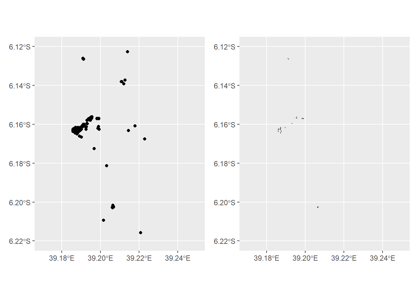
We can visualise the retrieved data about hotels in Unguja using the ggplot2 package. We can easily visualise simple feature objects using the geom_sf() function of ggplot2.
points = hotels$osm_points
polygons = hotels$osm_polygons
hotels.points = ggplot()+
geom_sf(data = points)+
coord_sf(xlim = c(39.17, 39.25),ylim = c(-6.22,-6.12))
hotels.poly = ggplot()+
geom_sf(data = polygons)+
coord_sf(xlim = c(39.17, 39.25),ylim = c(-6.22,-6.12))
hotels.points + hotels.poly
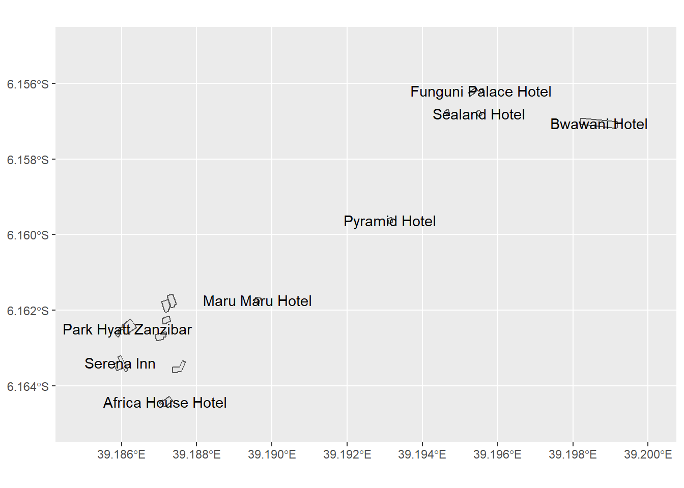
ggplot(data = polygons)+
  geom_sf()+
  coord_sf(xlim = c(39.185, 39.20),ylim = c(-6.165,-6.155))+
  geom_sf_text(aes(label = name),check_overlap = TRUE)+
  theme(axis.title = element_blank())
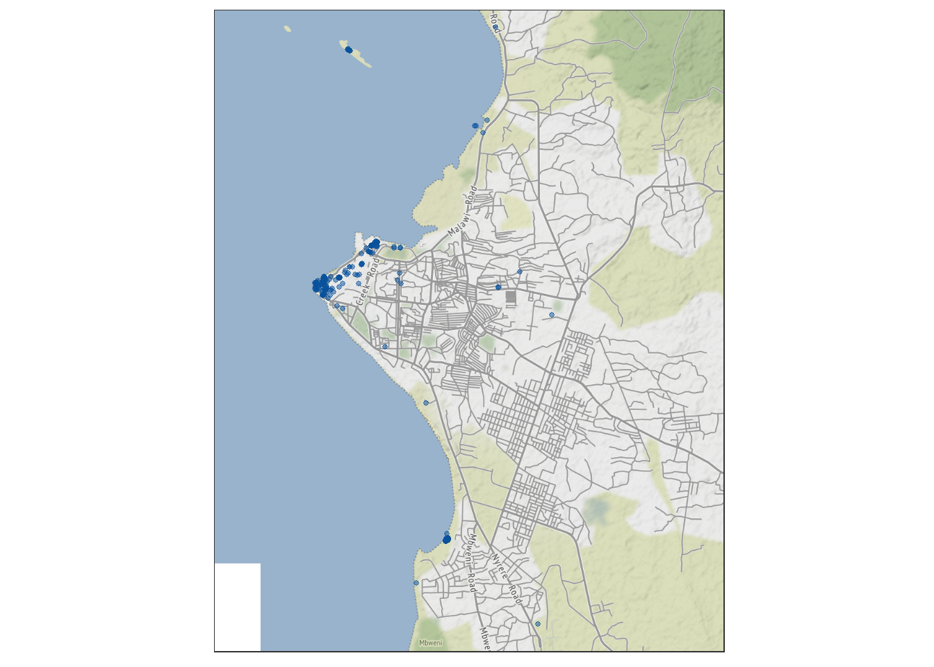
While the visualisation above provides useful information about the spatial distribution of hotels in Unguja Island, we can make it the aesthetic more appealing by overlying hotel locations with basemaps. For this we use the ggmap package. To get a map of Unguja, we use the
get_map() function provided by the ggmap package. Here we have used the maptype “roadmap”, but the function allows many more map types which can be found here.
aoi = c(left = 39.17, bottom = -6.22, right = 39.25, top = -6.12)

unguja_basemap = get_map(location = aoi, maptype = "roadmap")
ggmap(ggmap = unguja_basemap) +
geom_jitter(data = points %>% wior::point_tb(),
aes(x = lon, y = lat),
colour = "#08519c",
fill = "#08306b",
alpha = .5,
size = 1)+
theme_bw() +
theme(axis.title = element_blank(), axis.text = element_blank(), axis.ticks = element_blank())
require(tmap)
tmap_mode(mode = "view")

tm_shape(shp = points)+
  tm_symbols(size = 0.02, col = "red", alpha = 0.1)
Conclusion
The osmdata package can also be used to download other spatial features such as shiplanes, and overlay them on top of each other using ggplot2 to create a map of Lagos. For this we create multiple queries for each feature as follows.

