Access altitude data and plot topograhy in R
Elevation data is used for a wide array of applications, including, for example, visualization, hydrology, and ecological modelling. There are several sources for digital elevation models such as the Shuttle Radar Topography Mission (SRTM), the USGS National Elevation Dataset (NED), Global DEM (GDEM), and others. Each of these DEMs has pros and cons for their use. Prior to its closure in January of 2018, Mapzen combined several of these sources to create a synthesis elevation product that utilizes the best available elevation data for a given region at given zoom level. Additionally, the elevation data are enhanced with the inclusion of bathymetry in oceans from ETOPO1.
In this post, I will take you through a process on how you can use a getData function from raster package (Hijmans 2017) to access and download the dataset to a specific geographical area. Let’s first load the packages we need.
library(tidyverse)
# library(raster)
# library(rnaturalearth)
# library(maps) #get city lat longs
library(ggrepel)
library(oce)
raster package has nifty funtion that allows us to define some parameters and download the dataset. For this case, I am interested to download the elevation dataset but only cover the geographical boundary of the country. To achieve that, I have to parse the country="Tanzania", mask=TRUE arguments in the cunction as the chunk below shows;
tz_raster = raster::getData(name = 'alt',
                            country="Tanzania",
                            mask=TRUE)

tz_raster
class : RasterLayer
dimensions : 1308, 1356, 1773648 (nrow, ncol, ncell)
resolution : 0.008333333, 0.008333333 (x, y)
extent : 29.2, 40.5, -11.8, -0.9 (xmin, xmax, ymin, ymax)
crs : +proj=longlat +datum=WGS84 +no_defs
source : TZA_msk_alt.grd
names : TZA_msk_alt
values : -1, 5778 (min, max)We notice that a raster dataset contain values ranges from -1 to 5778. We need to know those cells with values less than 1, which is bathymetry and then remove them from our dataset
tz_raster[tz_raster < 1] [1] 0 0 0 0 0 0 0 0 -1 -1 0 -1 0 0 0 0 0 0 0 0 0 0 -1 0 0
[26] 0 0 0 0 0 0 0 0 0 0 0 0 0 0 0 0 0 0 0we notice that there are only four cell, then we assign them a values of NA
tz_raster[tz_raster < 1] = NA
tz_raster
class : RasterLayer
dimensions : 1308, 1356, 1773648 (nrow, ncol, ncell)
resolution : 0.008333333, 0.008333333 (x, y)
extent : 29.2, 40.5, -11.8, -0.9 (xmin, xmax, ymin, ymax)
crs : +proj=longlat +datum=WGS84 +no_defs
source : memory
names : TZA_msk_alt
values : 1, 5778 (min, max)My plotting package in this post is ggplot2 (Wickham 2016), which required the data structured in rectangular format of rows (records) and column (variable) commonly known as data.frame. Therefore, to plot elevation data in ggplot requires me to convert raster dataset into data frame. Thank Hijmans (2017) for inclusion of as.data.frame function that convert the raster into data frame in single line of code.
tz.raster.df = tz_raster %>%
  raster::as.data.frame(xy = TRUE) %>%
  drop_na() %>%
  rename(lon = 1, lat = 2, altitude = 3)

tz.raster.df %>%
  dplyr::sample_n(size = 5)
lon lat altitude
1 38.77917 -4.754167 380
2 31.12917 -8.229167 1269
3 30.46250 -3.887500 1185
4 33.05417 -6.112500 1151
5 37.51250 -7.062500 1068The other sources of data I need is the cities across the country that a populous. To obtain this dataset, I have to extract from maps package, which has a dataset contain the world cities. Therefore, I access the world.cities dataset and then filtered it to cities that are within the Tanzania and then pick ten cities that are populous. The chunk below hightlight the code used to obtain the populous cities in Tanzania.
populous.cities = maps::world.cities %>%
  filter(country.etc == "Tanzania") %>%
  top_n(n = 10, wt = pop)

populous.cities
name country.etc pop lat long capital
1 Arusha Tanzania 362904 -3.36 36.67 0
2 Dar es Salaam Tanzania 2805523 -6.82 39.28 0
3 Dodoma Tanzania 188150 -6.17 35.74 1
4 Kigoma Tanzania 171206 -4.88 29.61 0
5 Mbeya Tanzania 304155 -8.89 33.43 0
6 Morogoro Tanzania 261424 -6.82 37.66 0
7 Moshi Tanzania 161246 -3.34 37.34 0
8 Mwanza Tanzania 458070 -2.52 32.89 0
9 Tanga Tanzania 230369 -5.07 39.09 0
10 Zanzibar Tanzania 422300 -6.16 39.20 0The populous cities is data frame, and contains geographical positions (long, lat), which i used to create a simple feature as shown below;
populous.cities.sf = populous.cities %>%
  st_as_sf(coords = c("long", "lat"), crs = 4326)
Then define color codes for ocean (bathymetry) and land (topography)
## test GMT colours as suggested by
## http://menugget.blogspot.ca/2014/01/importing-bathymetry-and-coastline-data.html
ocean.pal <- colorRampPalette(c("#000000", "#000209", "#000413", "#00061E",
    "#000728", "#000932", "#002650", "#00426E", "#005E8C", "#007AAA", "#0096C8",
    "#22A9C2", "#45BCBB", "#67CFB5", "#8AE2AE", "#ACF6A8", "#BCF8B9", "#CBF9CA",
    "#DBFBDC", "#EBFDED"))
land.pal <- colorRampPalette(c("#336600", "#F3CA89", "#D9A627", "#A49019", "#9F7B0D",
    "#996600", "#B27676", "#C2B0B0", "#E5E5E5", "#FFFFFF"))
We also need the basemap of Africa shapefile
africa = st_read("d:/semba/Deep sea/data/africa.shp", quiet = TRUE) %>%
  mutate(name = stringr::str_to_upper(CNTRY_NAME)) %>%
  filter(name != "TANZANIA")
The code in the chunk below was used to map the elevation data in Tanzania shown in figure 1
ggplot()+
  geom_raster(data=tz.raster.df,
              aes(x=lon,y=lat,fill=altitude))+
  scale_fill_gradientn(colours = land.pal(n = seq(100, 6000, by = 50)),
                       # trans = scales::sqrt_trans(),
                       name = "Altitude (m)",
                       guide = guide_colorbar(barwidth = unit(.4, "cm"), barheight = unit(6, "lines")))+
  geom_sf(data = populous.cities.sf, shape = 21, fill="white", color="grey20" )+
  geom_sf(data = africa)+
  geom_sf_text(data = africa, aes(label = name), check_overlap = TRUE)+
  geom_text_repel(data=populous.cities,aes(x=long,y=lat,label=name))+
  coord_sf(xlim = c(29.5,40.5), ylim = c(-12,-1) )+
  theme_bw()+
  theme(axis.title = element_blank(), legend.position = c(.1,.16), legend.background = element_rect(fill = "white", colour = "black", size = .5))+
  labs(caption="Data from STRM | Chart @semba",
       # title="THE TOPOGRAPHY | BONGO",
       # subtitle="Altitude map of Tanzania. Altitude expresesed in meters.",
       fill="Altitude (meters)")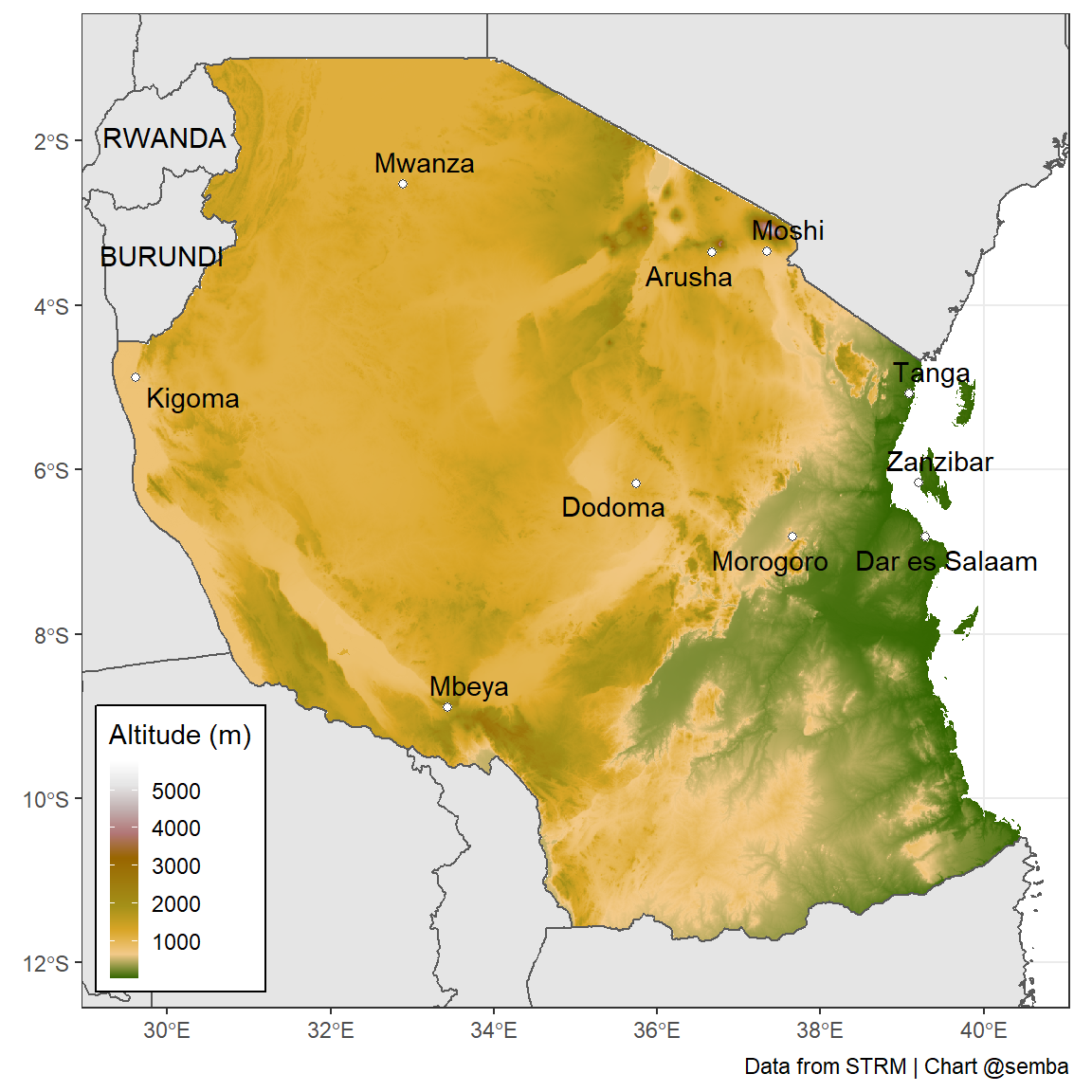
Figure 1: Topography of Tanzania
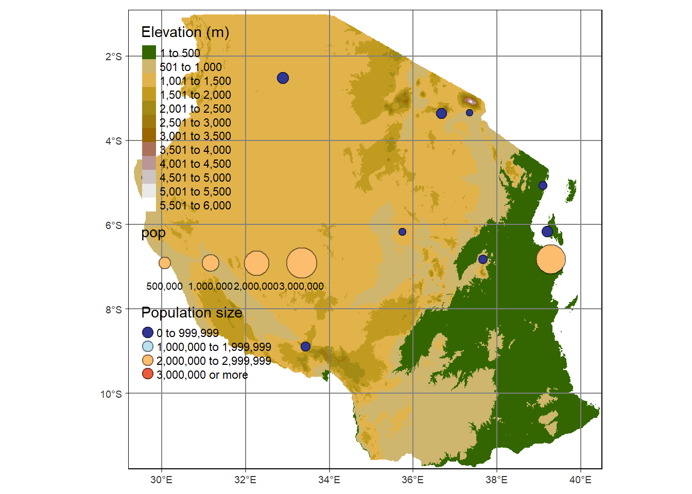
and a bonus is an interactive map of the elevation of Tanzania and population size of the cities
require(tmap)
tmap_mode(mode = "view")

tm_shape(shp = tz_raster, name = "Elvation (m)")+
  tm_raster(palette = land.pal(n = seq(100, 6000, by = 50)), n = 10,
            title = "Elevation (m)") +

  tm_shape(shp = populous.cities.sf)+
  tm_bubbles(size = "pop", scale = 2,
             col = "pop",
             border.col = "black", border.alpha = .5,
             style="fixed", breaks=c(seq(0, 3000000, by=1000000), Inf),
             palette="-RdYlBu", contrast=1,
             title.col="Population size") +
  tm_format("World")
tmap_mode(mode = "plot")
tm_shape(shp = tz_raster, name = "Elvation (m)")+
tm_raster(palette = land.pal(n = seq(100, 6000, by = 50)), n = 10,
title = "Elevation (m)") +
tm_shape(shp = populous.cities.sf)+
tm_bubbles(size = "pop", scale = 2,
col = "pop",
border.col = "black", border.alpha = .5,
style="fixed", breaks=c(seq(0, 3000000, by=1000000), Inf),
palette="-RdYlBu", contrast=1,
title.col="Population size") +
tm_layout(frame = TRUE)+
tm_graticules(ticks = TRUE)