Text Mining and Wordcloud in R
Word clouds
Word clouds visualize word frequencies of either single corpus or different corpora. Although word clouds are rarely used in academic publications, they are a common way to display language data and the topics of texts - which may be thought of as their semantic content. To exemplify how to use word clouds, we are going to have a look at the State of Environment issued in 2019 by the department of environment of the vice president’s office. We first load the packages that we are going to use during the session,
require(ggwordcloud)
require(magrittr)
require(tidyverse)
require(tidytext)
require(wordcloud)
require(RColorBrewer)
require(magrittr)

pal <- brewer.pal(8,"Dark2")
In a first step, we load and process the data as the relevant packages are already loaded.
After loading the data, we need to clean it.
Since the document is in pdf, we are goingt to use pdf_data function from **pdftools* package
soe = pdftools::pdf_data(pdf = "d:/semba/vpo/vpo reports/STATE OF THE ENVIRONMENT THIRD REPORT.pdf")We then process the text and compute frequency of occurance of each word
soe.txt = soe[c(1:194)] %>%
  bind_rows() %>%
  select(text) %>%
  mutate(txt.length = str_length(text)) %>%
  filter(txt.length > 4) %>%
  group_by(text) %>%
  count(sort = TRUE) %>%
  ungroup()
After the data is processed, we can now create word clouds. However, there are different word clouds:
- (Common) word clouds
- Comparative clouds
- Commonality clouds
Common or simple word clouds simply show the frequency of word types while comparative word clouds show which word types are particularly overrepresented in one sub-corpus compared to another sub-corpus. Commonality word clouds show words that are shared and are thus particularly indistinctive for different sub-corpora. Then we plot with ggwordcloud package
soe.txt %$%
  ggwordcloud::ggwordcloud(words = text,
                           freq = n,
                           random.order = FALSE,
                           max.words = 100,
                           colors = pal)
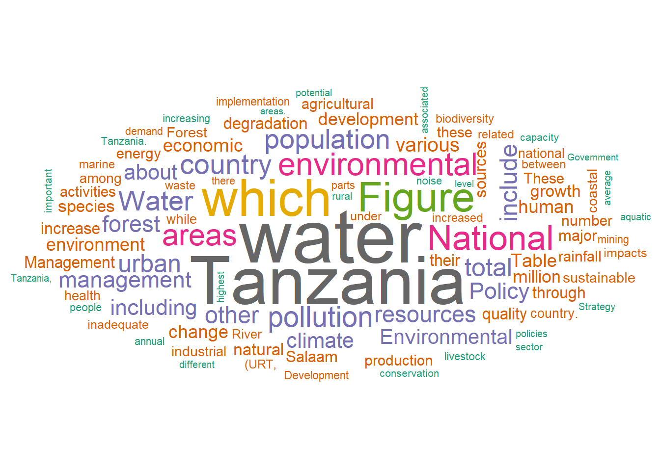
Figure 1: Wordcloud of of the State of Environment 2019 processed and drawn with ggwordcloud. However, notice that the punctuations and white space on the plot
We notice that the plot contain some of the punctuation words, which are not required. Hence, we switch to the other approach that would address the challenge of white spaces, punctuations and …..First this required text, we read and import the file as the chunk below hightlight
txt = read_tsv(file = "d:/semba/vpo/vpo reports/STATE OF THE ENVIRONMENT THIRD REPORT.txt")Once the dataset is imported into the session, we ought to clean it.
doc = txt %>%
  tm::VectorSource() %>%
  tm::Corpus() %>%
  # clean text data
  tm::tm_map(tm::removePunctuation) %>%
  tm::tm_map(tm::removeNumbers) %>%
  tm::tm_map(tolower)  %>%
  tm::tm_map(tm::removeWords, tm::stopwords("english")) %>%
  tm::tm_map(tm::stripWhitespace) %>%
  tm::tm_map(tm::PlainTextDocument)
Then plot with wordcloud package
# load package
library(wordcloud)

# create word cloud
wordcloud(words = doc, max.words = 120,
          colors = pal, min.freq = 20,
          random.order = FALSE)
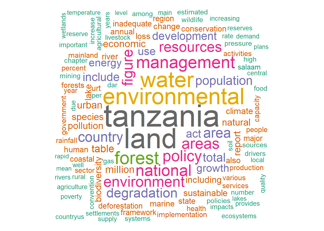
Figure 2: Wordcloud of of the State of Environment 2019 processed and drawn with wordcloud package
However, we notice that the plotting device of worldcloud does not give us an appealing picture. We can switch to ggcloudword package. Unfortunately, the package does not work on format other than data frame. We first need to convert the dataset into data frame and split the words in a sentense into single words using str_split function from stringr package
doc2 = doc$content$content %>%
  as_tibble() %>%
  stringr::str_split(pattern = " ") %>%
  as.data.frame() %>%
  rename(text = 1)

doc2 %>%
  head()
text
1 cvice
2 presidents
3 office
4 government
5 city
6 pThen group the word and compute the frequency of each word
doc.group = doc2 %>%
  group_by(text) %>%
  count() %>%
  arrange(desc(n)) %>%
  ungroup()

doc.group
# A tibble: 3,558 x 2
text n
<chr> <int>
1 tanzania 254
2 land 228
3 environmental 176
4 water 171
5 forest 130
6 management 125
7 national 113
8 policy 109
9 areas 107
10 environment 103
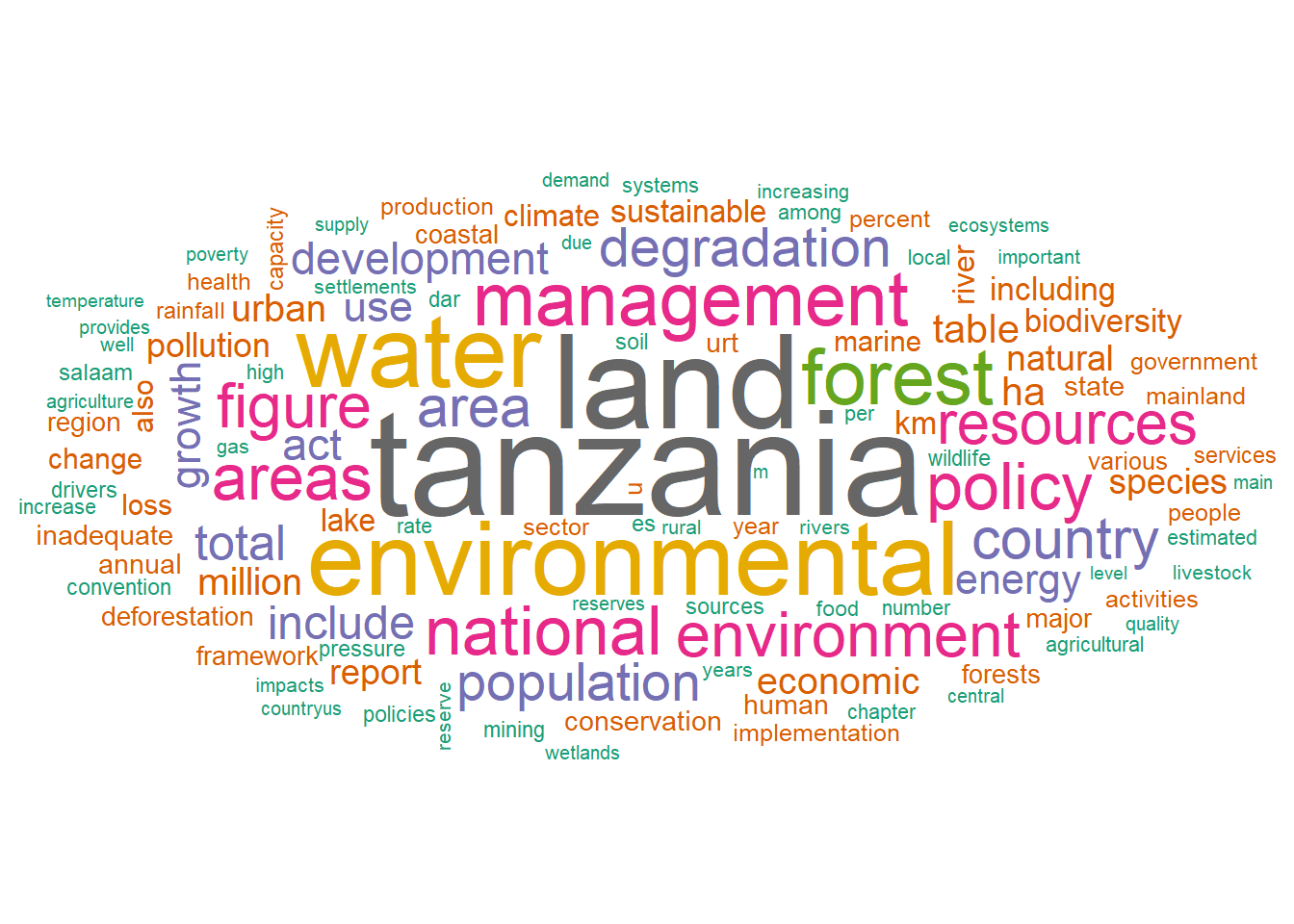
# ... with 3,548 more rowsOnce we have the dataset ready, we can plot with ggworldcloud. The figure 3 display
doc.group%$%
  ggwordcloud::ggwordcloud(words = text,
                           freq = n,
                           random.order = FALSE,
                           max.words = 120,
                           colors = pal)
Figure 3: Wordcloud of of the State of Environment 2019 processed and drawn with ggwordcloud

